


When getting acquainted with a new FEA software, solving pre-defined computational examples is a straightforward way to validate the computational method and the way of building up the model. This post summarizes one such validation process, which have been acquired during the examination of the possible applications of an open-source FEA environment: code_aster (being run under Salome Meca).
The example solved (‘Hemisphere – Point Load’ benchmark found in ’The Standard NAFMES Benchmarks’ published by NAFEMS Ltd.) defines a hemispherical shell being pushed and pulled simultaneously (figure 1). The hemisphere has a mid-surface radius of 10 [m] and thickness of 0.04 [m]. The load is 2 [kN] applied on points according to figure 1. Exploiting the symmetries, a quarter model is used for the solution.
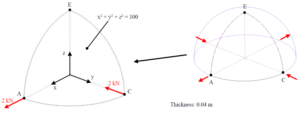
figure 1 – problem definition and the model.
According to the theory described by Morley and Morris (Morley, L.S.D. and Morris, A.J. – Conflict Between Finite Elements and Shell Theory, Procs. 2nd World Congress on Finite Elements: Finite Elements in the Commercial Environment, pages 532-561. 1978.), the solution of the problem (the displacement to the radial direction), which considers membrane effects, inextensional bending and edge effects can be written as
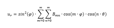
where ur is the radial deflection, θ is the angle measured about the vertical axis and φ is the angle measured in a plane radial to the axis of the hemisphere. Bmn are constants. With the given properties, the radial displacement of point A is
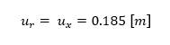
which gives us the target value.
Despite the forces applied, displacement boundary conditions are also considered while building up the simulation model. The z displacement of point E is considered to be zero, while symmetrical boundary conditions are applied on edges AE and CE. Isotropic material model is defined with E = 68.25∙103 [MPa] and ν = 0.3 [-]. Shell elements are used for the computation.
Table 1 summarizes the results for different number of elements (element sizes determined by the number of elements distributed along the edges of the geometry). A displacement plot is shown of figure 2.
table 1 – result of the simulations.
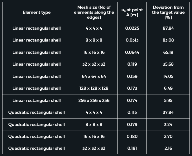
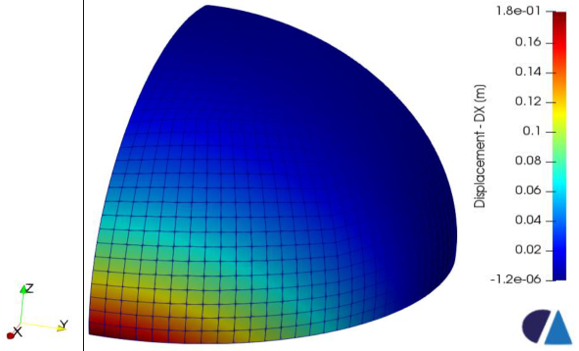
figure 2 – x directional displacement plot (quadratic rectangular shell, size: 32 x 32 x 32).
The animation below summarizes the core ideas and steps of the simulation, while also showing the deformed shape.
The above described process was (and still is) a good opportunity for us to research the possibilities of using open source finite element enviroments for computational tasks, thus creating cheaper, but still professional solutions for our customers.