
The VDI 2230 Guideline
2021.06.16.
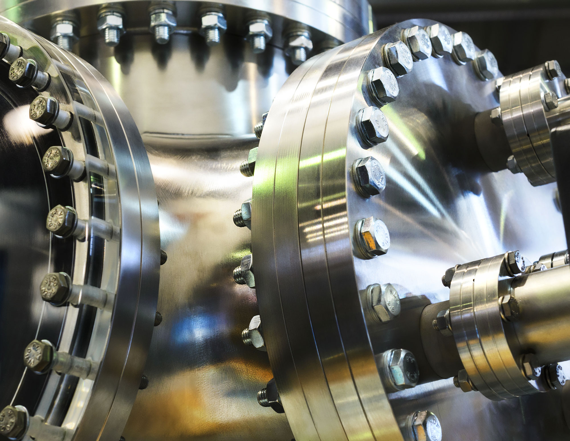
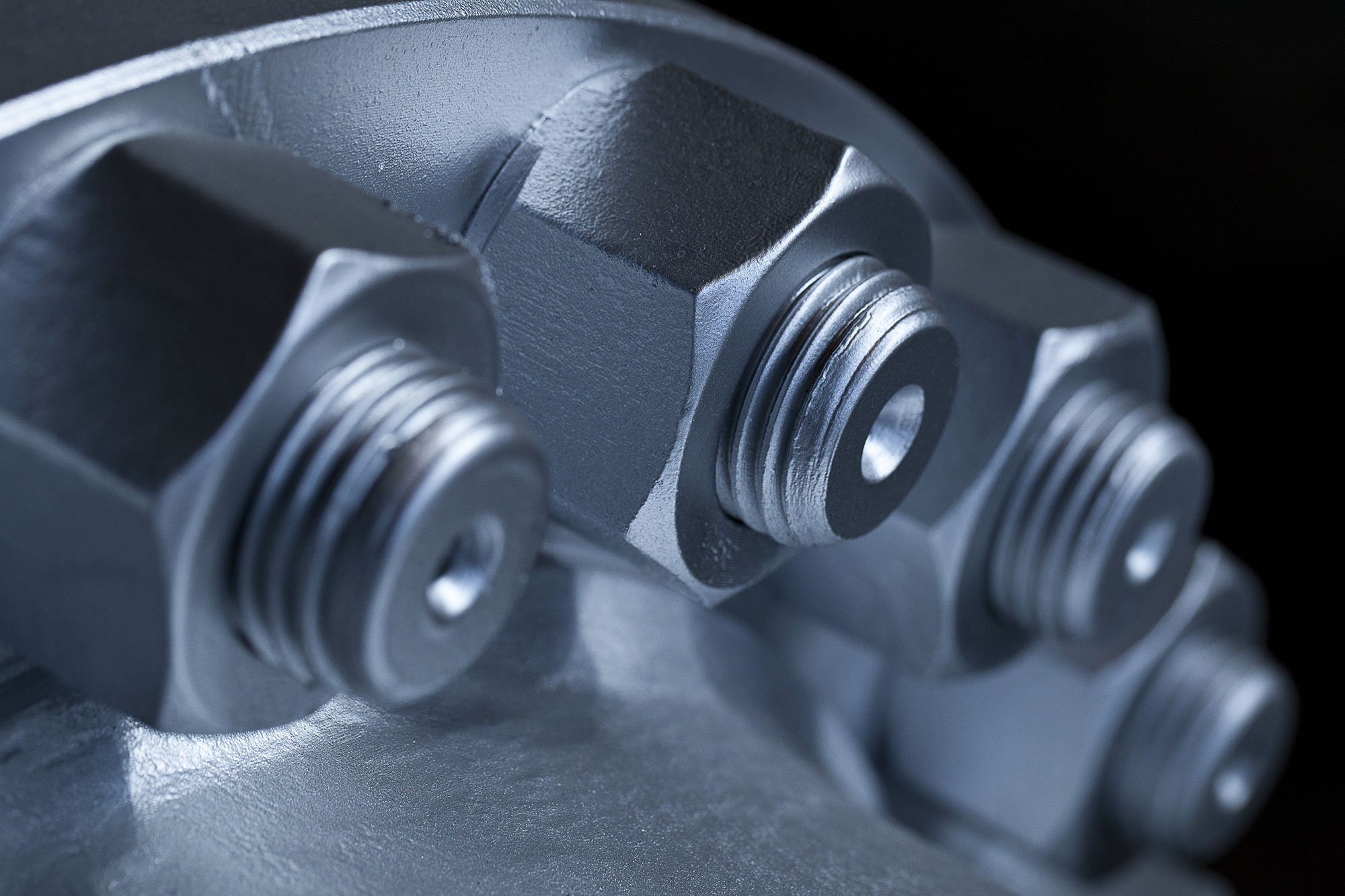
Whoever has ever wanted to size a screw must have met the term VDI, which is the association of German engineers (Verein Deutscher Ingenieure) and their guidelines for sizing bolted joints is the VDI2230. It is not just an enjoyable read, but it is worth taking the trouble and solving some sample exercises from it. We did it with the crank of an internal combustion engine, what’s more, in parallel we analysed it also using FE, because we were interested how simulation and analytical results correlate. In our experience, the simplified analytical method works well in the case of the complex geometry of a bolted screw as well. The load diagrams of the joint determined in analytical way and using FE technique as well as the changes in the graphs due to external loading were similar to each other. Our blog post about the joint diagram can be found here. Please note that in the fatigue of the bolting the stress amplitude, caused by the cyclic external load, is of vital importance. Although on the joint diagram the FEM and analytical results seem to be almost the same, the fatigue causing stress amplitude in simulation can differ with 100% from the result calculated on paper. We could decide which method provides more reliable estimation after series of experiments. The engineer’s intuition tells us that the simulation is the closest to the real practice.
The joint diagram
One of the most exciting graphs in the engineering. It shows at the same time the compression of the clamped elements and the elongation of the screw, shifting them on the horizontal axis so that they cross each other at maximum pre-load. Supposing that due to external load the screw and the compressed elements share this load in the same proportion, as much the elongation of the screw grows as much the compression of clamped elements decreases (into minus). It is easy to illustrate the effect of the external load on the joint by the elongation of the line in the diagram which represents the compliance of the screw. The cyclicality of the external load causes repetitive stress and strain. It can be easily accepted that it is essential to define the exact stiffness and resilience of the screw and the compressed elements to be able to calculate the exact impact of the stress/fatigue load. Since the amplitude that we are looking for is only a small part of the pretension force, only a small change in the applied parameters can have a huge impact on the screw’s estimated strength. It can be seen in the case of finite element simulations as well that a small change of the iteration interval is enough to calculate a different lifespan to the same bolt on the same model, with the same load. One of the reasons is friction, which you can read about here. Considerable experience is necessary to conduct reliable analytical calculations and FE simulations on bolted joints.
Bolts and friction

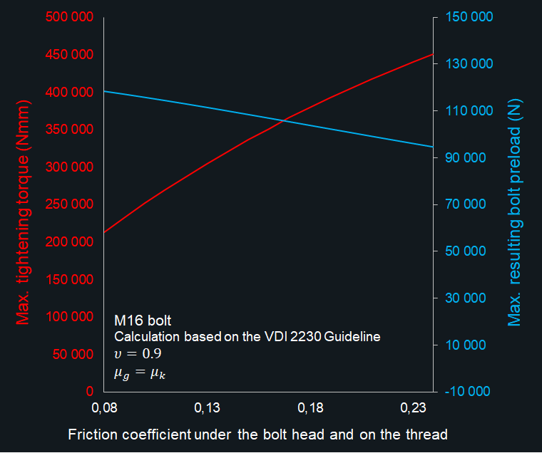
The bolted joint is a force-locking joint type, and this is why we like it so much, it is releasable, reusable within its lifespan, robust, and easy to use. Unfortunately, it is also the force- locking itself, which causes the most challenges. In the case of force-locking binding the friction force ensures the self-locking. The friction, however, can cause some problems in practice. From engineering point of view the most problematic characteristic of friction is its non-permanent value (coefficient of friction). In addition to this, in engineering we can calculate mostly with the Coulomb friction model, which means that we cannot define the exact range of the slip, when the sliding appears at the interface. We can only estimate the range of this slip. Moreover, the size of this range depends on the coefficient of the friction. The higher the friction coefficient, the wider the range is, and the higher extremes we have to consider. Of course we have the same problem when realizing the tightening of the bolts during bolt mounting. In the calculations the different bolt tightening tools are considered with different parameters standing for the uncertainties of the special tools and methods (wrench, manual torque wrench, pneumatic torque wrench, tightening for angle, etc…) If the coefficient of friction is high it can be problematic, because it means a significant torque will appear in the bolt limiting the applicable pretension force. See the diagram below. Defining the impact of the friction using the finite element method is not obvious at all (here you can find the relevant blog post).
Introduction to bolted joints

One of the most popular machine elements, in terms of its operational background, it is a simple slope. Most of the machines contain it, everybody uses it. Even though no other joint type has been researched so widely, engineers can only estimate the performance of a bolted joint, due to-among others- the endless number of practical, non-textbook cases such as: bolts stressed to the yield point, pretension in aluminium, setting on paint films, etc. When we analyse the strength of the bolting, we have to take into consideration more parameters at the same time, and it is not easy to find our way among the relevant standards, recommendations and dimensioning specifications (e.g. VDI2230 see our later blog posts) in light of the field experiences. Finite element analysis is not always necessary to assess a bolt connection, but it might be helpful to define the loading of the bolt and estimate its safety and utility. In the following posts we discuss some topics about bolted joints and highlight some factors, which define (being unclear to most of us) the behaviour of a certain joint.
Karman vortex shedding
2021.06.11.
Laminar flow around a 2D cylinder – Kármán vortex shedding
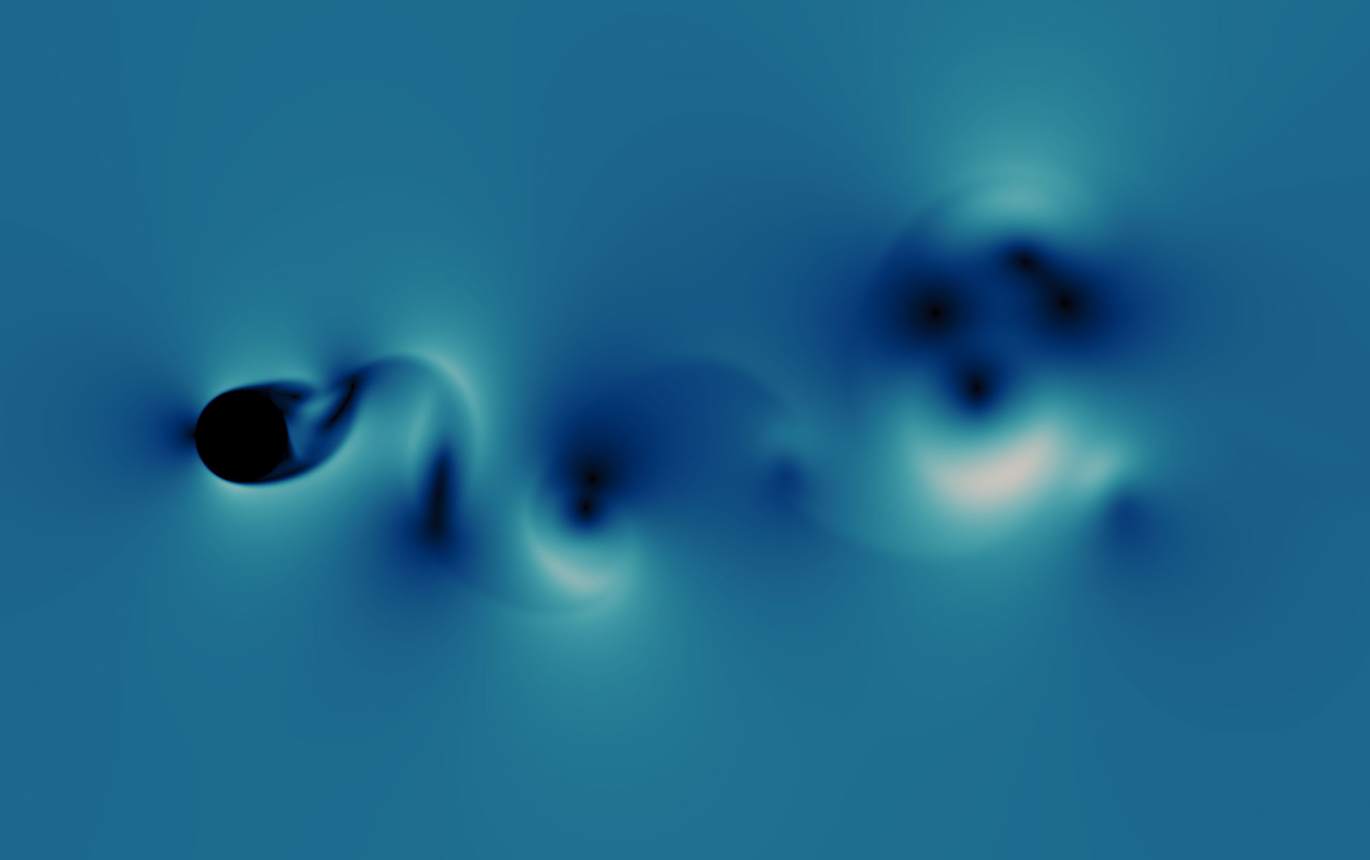
Low Reynolds number flows around a cylinder is one of the most well-known, and most investigated cases in Computational Fluid Dynamics (CFD). It is probably due to the interesting phenomenon that can occur in this type of flow, the Karman vortex shredding.
Around Re 90-150 the fluid behind the cylinder starts to produce vortexes with periodically opposite orientations. The phenomenon became a great benchmark and validation case, considering the simplicity of the geometry combined with the complex behaviour of the flow.
The purpose of this study is to investigate the effect of different meshing methods on the solution accuracy.
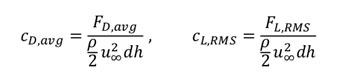
The lift- (CL) and drag coefficients (CD) were investigated on a 2D cylinder using OpenFOAM. Since these are time dependent – oscillating values, an average was calculated for the drag- and a root mean square for the lift coefficient using the following formulas:
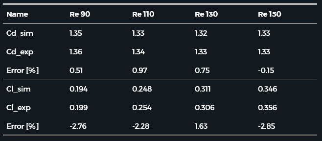
Flow with four different Re numbers (from 90-150) was examined. The investigations of Henderson and Norberg were considered as the target, the reference data is summarised in the table below.
Table 1. Experimental data for the cylindrical bodies

Air was used in the analyses, in order to accurately recreate the experimental environment. To maintain low Re numbers. we had to set our inlet velocity ranging from 0.0073 m/s to 0.022 m/s. The length of the wind tunnel was 10 meters, and the height was 8 meters. The model setup is displayed in the following sketch.
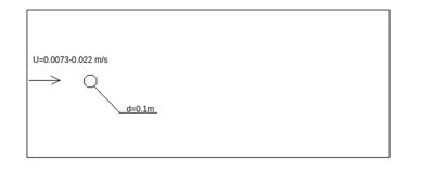
Figure 1. Model setup.
Since the simulation was laminar and transient, OpenFOAM’s icoFoam solver was used for the analysis. The initial mesh was generated with Salome Meca’s Netgen module. The prism-dominant (extruded triangles) mesh with the use of viscous sublayers consisted of 81 000 cells and can be seen in the pictures below.
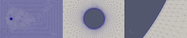
Figure 2. CFD mesh generated by Salome Meca’s Netgen module consisting of 81 000 cells.
Table 2. summarises the simulation result lift- (CL) and drag coefficients (CD) compared with the experimental results. The simulation results seem accurate based on the comparison.
Table 2. Lift- and drag coefficient around a 2D cylinder at Re 90-150.
The following animation shows the laminar vortex shedding at Re = 150:
A further mesh convergence study was made, to find more efficient approaches to solve this problem.
Fully hexahedral meshes were investigated generated by OpenFOAM’s blockMesh utility. Four refinement levels were made, both with Salome and blockMesh. These meshes are displayed in the following Figures.
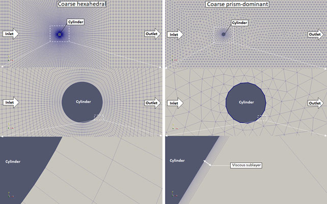
Figure 3. Coarse meshes generated with snappyHexMesh (left) and Salome Meca (right)
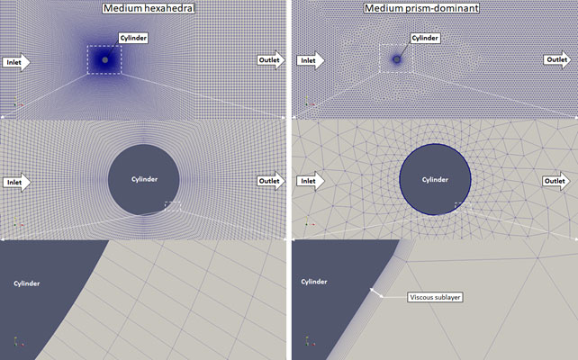
Figure 4. Medium meshes generated with snappyHexMesh (left) and Salome Meca (right)
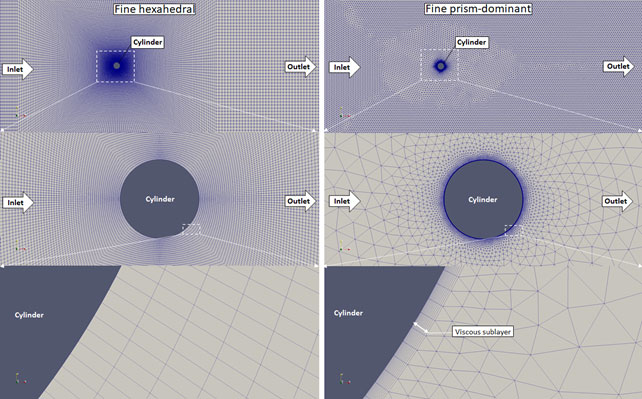
Figure 5. Fine meshes generated with snappyHexMesh (left) and Salome Meca (right)
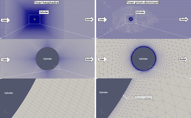
Figure 6. Finer meshes generated with snappyHexMesh (left) and Salome Meca (right)
The meshes displayed in Fig. 3-6. were used to run the scenario at a Reynolds number of 150. For these simulations the wind tunnel height was decreased to 3 meters, because it seemed to be perfectly enough for the flow to develop undisturbedly. The Salome generated meshes were labelled with “sm” initials whereas the blockMesh generated ones got the “bm” label.
An animation of the vortex shredding forming in each case.
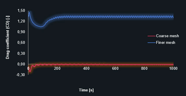
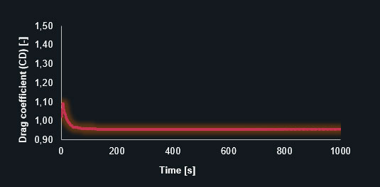
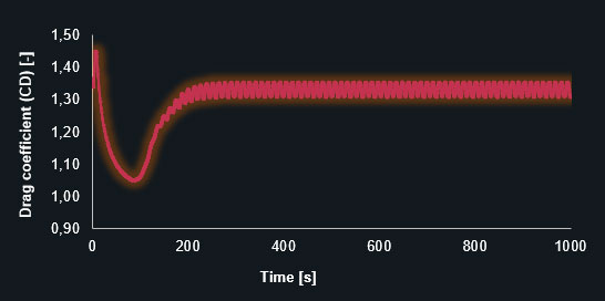
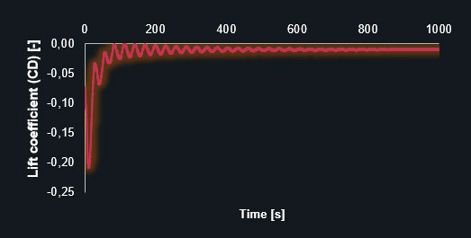
And also diagrams of the lift- (CL) and drag coefficients (CD) in each timestep, on the coarse and finer prism-mesh.
Drag coefficient (CL) in a coarse and finer prism-dominant mesh
Drag coefficient (CD) – coarse prism-dominant mesh
Drag coefficient (CD) – fine prism-dominant mesh
Lift coefficient (CL) – coarse prism-dominant mesh
Lift coefficient (CL) – fine prism-dominant mesh
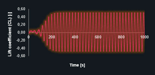
The diagrams clearly show that the finer mesh produces the expected oscillating results for the lift and drag coefficients. The simulation with the coarse mesh converges to a discrete value leading to an inaccurate solution. The following table contains the results in detail.
Table 3. Comparison of the different meshing methods at different refinement levels
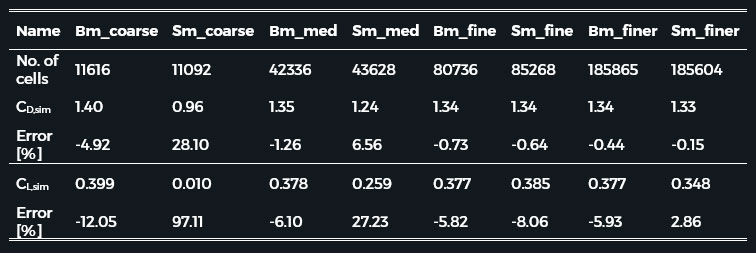
As the results show the hexahedral mesh can produce more accurate results with the same number of cells. But nevertheless, at the end, the Salome prism-dominant mesh gave the best result. This is probably due to the added viscous sublayers and the considerably finer mesh around the cylinder.
The animation also shows that the prism meshes that converged, converged much faster than the hexahedral ones. (Although the simulation with the coarse mesh didn’t even started the vortex shedding.)
Generally speaking, a blockMesh generated mesh leads to precise and fast results. In case one needs even more precision, it is worth using a finer mesh and viscous sublayers.